NURBS Formats in APT Output | ||||
|
| |||
Fixed Axis and Variable Axis NURBS Statements
You can generate NC output files containing tool motion descriptions using a format based on NURBS technology for both fixed or variable axis programs. This format is recognized by most new generation NC controllers (such as the Siemens 840D). It supports High Speed Milling (HSM) in order to reduce machining time and improve surface quality. Examples of Fixed Axis and Variable Axis NURBS output statements that can be found in the generated APT file are given below.
Examples
- Fixed Axis NURBS example
BEGIN NURBS_SIEMENS(D=3,F=4000,AXIS=0.00,0.00,1.00);
N0,XT= 0.000,YT=0.000,ZT=0.000,DK= 0.00,W=1.0;
N1,XT=10.000,YT=0.000,ZT=0.000,DK= 0.00,W=1.0;
N2,XT=20.000,YT=0.000,ZT=0.000,DK=30.00,W=1.0;
N3,XT=30.000,YT=0.000,ZT=0.000,DK= 0.00,W=1.0;
END NURBS;
- Variable Axis NURBS example
BEGIN NURBS_SIEMENS(D=3,F=4000,AXIS=VAR,LENGTH=100.00);
N0,XT= 0.000,YT=0.000,ZT=0.000,XH= 0.000, $
YH=0.000,ZH=100.00,DK= 0.00,W=1.0;
N1,XT=10.000,YT=0.000,ZT=0.000,XH=10.000, $
YH=0.000,ZH=100.00,DK= 0.00,W=1.0;
N2,XT=20.000,YT=0.000,ZT=0.000,XH=20.000, $
YH=0.000,ZH=100.00,DK=30.00,W=1.0;
N3,XT=30.000,YT=0.000,ZT=0.000,XH=30.000, $
YH=0.000,ZH=100.00,DK= 0.00,W=1.0;
END NURBS;
These statements are supported by some of the Post-Processors proposed under Output for conversion to Siemens Nurbs/Bspline statements.
![]()
Benefit Derived from Using NURBS Interpolated Tool Paths
There are several advantages in using NURBS interpolated tool paths:
- gain in overall dynamic performance,
- better surface quality,
- gain in productivity.
Gain in Overall Dynamic Performance
Because NURBS curves introduce C2 continuity in the path as
often as possible, it decreases dramatically the machine decelerations produced
by curvature discontinuities. This fact is easily explained. If the second
derivative of the curve is not continuous on a point, the numerical controller
detects a discontinuity in acceleration at this position. There are two
solutions to this problem:
- Let the acceleration go to its calculated value. Theoretically, this means that the variation of acceleration (which is called Jerk) in the neighborhood of this point can be infinite. In fact, the Jerk is directly linked to the power of the linear motors and the inertia of the machine. So it has a specified limit value (which is constant).
- Force the speed of the tool to a small value.
This means that the acceleration and the Jerk can be forced to a small
value. The machine has a big slowdown. This is the current method employed
by the numerical controller. This method had big disadvantages:
- First, a lot of machining time can be lost due to continuity problems.
- Second, a big feedrate variation during a machining operation can mark the surface being machined and so deteriorate surface quality.
Better Surface Quality
Compared to linear interpolation, a NURBS machined surface can have a smoother aspect and cannot provide a facettized result like in linear interpolation. A very good surface quality can be obtained without significantly reducing the program tolerance.
Gain in Productivity
NURBS output provides better dynamic properties and, as a result, the gain in productivity using NURBS instead of linear or linear/circular interpolation is increased. A comparison in terms of machining time gain of the different APT output formats has been verified with a lot of programs including 3-axis and 5-axis Machining Operations.
This interpolation provides as good results as the numerical controller polynomial interpolation. The advantage of using NURBS interpolation is that there is no need for extra numerical controller parameterization.
The NURBS toolpath final tolerance is equal to 1.5 times the computed operation tolerance.
![]()
APT Output Format
The fixed and variable axis NURBS output can be included in regular APT output containing other classes of 3 or 5 axis tool motion statements.
The most common of these statements are:
GOTO / x, y, z
GOTO / x, y, z, i, j, k
Example:
GOTO / 0.00000, 89.19372, 12.00000

GOTO / 0.00000, 89.19372, 12.00000, 0.000000, 0.000000, 1.000000
Syntax
A Fixed Axis NURBS for Siemens Output looks like this:
BEGIN NURBS_SIEMENS (D=3,F=8000.000,AXIS= 0.000000, 0.000000, 1.000000)
N0, XT= 0.00000, YT= 89.19372, ZT= 12.00000,DK=0.000,W=1.000;
N1, XT= -35.25923, YT= 82.30182, ZT= 12.00000,DK=0.000,W=1.000;
N2, XT= -70.67279, YT= 76.14709, ZT= 12.00000,DK=107.790,W=1.000;
N3, XT= -105.90481, YT= 69.14878, ZT= 12.00000,DK=0.000,W=1.000;
END NURBS
A Variable Axis NURBS for Siemens Output looks like this:
BEGIN NURBS_SIEMENS (D=3,F=8000.000,AXIS=VAR,LENGTH= 50.000)
N0, XT= -75.76597, YT= 71.65094, ZT= -21.94567, XH= -72.178223, YH=$
62.527376, ZH= 27.083796,DK=0.000,W=1.000;
N1, XT= -78.91003, YT= 71.01919, ZT= -21.77676, XH= -79.690819, YH=$
61.032142, ZH= 27.416003,DK=0.000,W=1.000;
N2, XT= -82.06101, YT= 70.37700, ZT= -21.56199, XH= -87.244248, YH=$
59.640659, ZH= 27.190920,DK=22.998,W=1.000;
N3, XT= -85.40313, YT= 69.68892, ZT= -21.29975, XH= -94.767915, YH=$
58.350206, ZH= 26.488684,DK=0.000,W=1.000;
END NURBS
Note:
- The number of digits used for each float value is not imposed.
- The $ character means that the instruction continues on the next line.
Mathematical and Geometrical Interpretation
| Instructions | Comments |
|---|---|
| D | Integer value Degree on the NURBS, means order-1, in most cases degree is 3 and order is 4. |
| F | Float value. Feedrate in mm per minute (Feedrate) |
| LENGTH | Float value. Distance (constant in the NURBS) between MT and MH control points. |
| N | Integer value. Rank of the control point in the NURBS, starts at 0 for the initial point. |
| XT, YT, ZT | Float values. Coordinates of the control point of the tool tip (MT). |
| XH, YH, ZH | Float values. Coordinates of the control point of a point on the tool axis (MH). |
| DK | Float value. Increment of nodal parameter related to this node (can be null, always >= 0.00). |
| W | Float value. Weight of the control point (in most cases it is set to 1.00 for all NURBS, which is Polynomial and not Rational in this case ). |
Let's consider this example: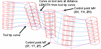
- You would note (DKi), (Wi), (XTi,YTi,ZTi), (XHi,YHi,ZHi) for all the values related to the control point i, for i in [0,NB]. With all this data, it is possible to define a NURBS function from [0.00,Kmax] to R6. Kmax = ΣDKi , for i=0 to NB.
- The nodal vector (U(I)) of the NURBS contains NB+5 Values: U(0)=0.00 U(1)=0.00 And for I=2 to NB+3 U(I)=U(I-1)+DK(I-2) (that is, U(2)=U(1)+DK(0)=0.00) then U(NB+4) = U(NB+3) = Kmax U(NB+5) = U(NB+4)
- In Fixed Axis mode, for each value of w in [0,Kmax], this function give 3 values: X(w), Y(w), Z(w), which are the control point coordinates of the tool tip at the w parameter.
- In Variable Axis mode, for each value of w in [0,Kmax], this function
give 6 values: XT(w), YT(w), ZT(w), XH(w), YH(w), ZH(w) which are the control
point coordinates of the points MT=(XT,YT,ZT) and MH=(XH,YH,ZH).
- MT is the position of the tool tip at the w parameter.
- MH is the position, at the w parameter, of the point on the tool axis located a distance LENGTH from MT.
- This length defines the active cutting part of the tool. This means that all transformations of the tool path must respect the machining tolerance (chordal deviation) for all points between MT and MH.
The first Tool position (XYZIJK) of the NURBS is:
X=XT0
Y=YT0
Z=ZT0
I=(XH0-XT0)/LENGTH
J=(YH0-YT0)/LENGTH
K=(ZH0-ZT0)/LENGTH.
![]()
Post Processing for Siemens 840D Format
Examples of formats used in Variable Axis Syntax and Fixed Axis Syntax are given below.
Variable Axis Syntax
The format used by 840D is the following.
BEGIN
NURBS_SIEMENS(D=3,F=xxxx,AXIS=VAR,LENGTH=100.00);
N0,XT=xt0,YT=yt0,ZT=zt0,XH=xh0,YH=yh0,ZH=zh0,DK=dk0,W=w0;
N1,XT=xt1,YT=yt1,ZT=zt1,XH=xh1,YH=yh1,ZH=zh1,DK=dk1,W=w1;
N2,XT=xt2,YT=yt2,ZT=zt2,XH=xh2,YH=yh2,ZH=zh2,DK=dk2,W=w2;
../..
Nn,XT=xtn,YT=ytn,ZT=ztn,XH=xhn,YH=yhn,ZH=zhn,DK=dkn,W=wn;
END NURBS;
If the previous block is a NURBS block:
SD=3 F xxxx ; NURBS degree and feedrate
Otherwise:
ORIVECT
G1 X Y Z A3=I B3=J C3=K ; first point of the NURBS, Control Point 0
Then:
ORICURVE
G642 ; start of continuous motion statement
BSPLINE SD=3 F xxxx ; NURBS declaration, degree and feedrate
X Y Z XH YH ZH PW=W PL=DK ; Control Point 1
X Y Z XH YH ZH PW=W PL=DK ; Control Point 2
../..
X Y Z XH YH ZH PW=W PL=DK ; Last Control Point of the NURBS.
Translation from V6 Format
All parameters are the same as the one on the corresponding V6 line (i), except for the first one. If needed it is translated by a G1 statement.
Siemens Xi= Catia XTI
Siemens Yi= Catia YTI
Siemens Zi= Catia ZTI
Siemens XHi= Catia XHi
Siemens YHi= Catia YHi
Siemens ZHi= Catia ZHi
Siemens PWi= Catia Wi
Siemens PLi= Catia DKi
APT Sample for Variable Axis NURBS
$$
-----------------------------------------------------------------

$$ Generated on Wednesday, September 25, 2002 05:24:47 PM
$$ APT VERSION 1.0
$$
-----------------------------------------------------------------

$$ Flank Mixed Combin
$$ Part Operation.1
$$*CATIA0
$$ Flank Mixed Combin
$$ 1.00000 0.00000 0.00000 0.00000
$$ 0.00000 1.00000 0.00000 0.00000
$$ 0.00000 0.00000 1.00000 0.00000
PARTNO Part Operation.1
FROM / 0.00000, 0.00000, 100.00000, 0.000000, 0.000000,
0.000000
PPRINT OPERATION NAME : Tool Change.10
$$ Start generation of : Tool Change.10
MULTAX
$$ TOOLCHANGEBEGINNING
CUTTER/ 8.000000, 4.000000, 0.000000, 4.000000, 0.000000,$
0.000000, 50.000000
TOOLNO/2,MILL, 8.000000, 4.000000,, 100.000000,$
60.000000,, 50.000000,4, 8000.000000,$
MMPM,15000.000000,RPM,CLW,ON,$
AUTO, 0.000000,NOTE
TPRINT/balld8,,balld8
LOADTL/2,2,2
$$ End of generation of : Tool Change.10
PPRINT OPERATION NAME : Multi-Axis Flank Contouring.2
$$ Start generation of : Multi-Axis Flank Contouring.2
FEDRAT/ 8000.0000,MMPM
SPINDL/15000.0000,RPM,CLW
BEGIN NURBS_SIEMENS (D=3,F=8000.000,AXIS=VAR,LENGTH= 50.000)
N0, XT= 19.75656, YT= 81.42861, ZT= 20.00000, XH= 19.757763,
YH=$
71.623025, ZH= 69.029078,DK=0.000,W=1.000;
N1, XT= 19.75625, YT= 83.94658, ZT= 7.40984, XH= 19.757454,
YH=$
74.140998, ZH= 56.438918,DK=0.000,W=1.000;
N2, XT= 19.75594, YT= 86.46456, ZT= -5.18032, XH= 19.757144,
YH=$
76.658971, ZH= 43.848757,DK=38.518,W=1.000;
N3, XT= 19.75563, YT= 88.98253, ZT= -17.77048, XH= 19.756835,
YH=$
79.176944, ZH= 31.258597,DK=0.000,W=1.000;
END NURBS
BEGIN NURBS_SIEMENS (D=3,F=8000.000,AXIS=VAR,LENGTH= 50.000)
N0, XT= 19.75563, YT= 88.98253, ZT= -17.77048, XH= 19.756835,
YH=$
79.176944, ZH= 31.258597,DK=0.000,W=1.000;
N1, XT= 19.38827, YT= 89.96343, ZT= -23.02431, XH= 19.389475,
YH=$
80.157844, ZH= 26.004770,DK=0.000,W=1.000;
N2, XT= 14.20175, YT= 89.85474, ZT= -27.41283, XH= 14.202952,
YH=$
80.049153, ZH= 21.616250,DK=15.662,W=1.000;
N3, XT= 9.00010, YT= 88.77303, ZT= -26.95061, XH= 9.001309,
YH=$
78.967440, ZH= 22.078468,DK=0.000,W=1.000;
END NURBS
../..
BEGIN NURBS_SIEMENS (D=3,F=8000.000,AXIS=VAR,LENGTH= 50.000)
N0, XT= 19.18055, YT= -42.44969, ZT= -6.28780, XH= 19.180191,
YH=$
-37.474471, ZH= 43.464058,DK=0.000,W=1.000;
N1, XT= 19.18049, YT= -41.57342, ZT= 2.47480, XH= 19.180128,
YH=$
-36.598205, ZH= 52.226657,DK=0.000,W=1.000;
N2, XT= 19.18042, YT= -40.69716, ZT= 11.23740, XH= 19.180065,
YH=$
-35.721939, ZH= 60.989257,DK=26.419,W=1.000;
N3, XT= 19.18036, YT= -39.82089, ZT= 20.00000, XH= 19.180002,
YH=$
-34.845674, ZH= 69.751856,DK=0.000,W=1.000;
END NURBS
$$ End of generation of : Multi-Axis Flank Contouring.2
FINISH
NC Code Sample for Variable Axis NURBS
N10 ;PROGRAMME : Part Operation.1
N20 ;PROGRAMMEUR: AAU
N30 ;DATE : AAU
G642
ffwon
N40 TRAORI
G57
M8
N50 ORIVECT
N60 G0 Z100.0
N70 G0 X0.0 Y0.0
N80 T2 M06
N90 G1 X19.75656 Y81.42861 Z20.0 A3=0.00002 B3=-0.19611
C3=0.98058
N100 ORICURVE
N110 G642
N120 BSPLINE SD=3 F8000.000
N130 X19.75625 Y83.94658 Z7.40984 XH=19.75745 YH=74.141 ZH=56.43892
PL=0.0
N140 X19.75594 Y86.46456 Z-5.18032 XH=19.75714 YH=76.65897
ZH=43.84876 PL=38.518
N150 X19.75563 Y88.98253 Z-17.77048 XH=19.75683 YH=79.17694
ZH=31.2586 PL=0.0
N160 X19.38827 Y89.96343 Z-23.02431 XH=19.38948 YH=80.15784
ZH=26.00477 PL=0.0
N170 X14.20175 Y89.85474 Z-27.41283 XH=14.20295 YH=80.04915
ZH=21.61625 PL=15.662
N180 X9.0001 Y88.77303 Z-26.95061 XH=9.00131 YH=78.96744
ZH=22.07847 PL=0.0
../..
N470 X19.19914 Y-42.982 Z-11.59413 XH=19.19878 YH=-38.00679
ZH=38.15773 PL=15.662
N480 X19.18055 Y-42.44969 Z-6.2878 XH=19.18019 YH=-37.47447
ZH=43.46406 PL=0.0
N490 X19.18049 Y-41.57342 Z2.4748 XH=19.18013 YH=-36.59821
ZH=52.22666 PL=0.0
N500 X19.18042 Y-40.69716 Z11.2374 XH=19.18007 YH=-35.72194
ZH=60.98926 PL=26.419
N510 X19.18036 Y-39.82089 Z20.0 XH=19.18 YH=-34.84567 ZH=69.75186
PL=0.0
N520 ORIVECT
N530 TRAFOOF
N540 G57
N550 M5 M9
N560 M30
Fixed Axis Syntax
The format used by 840D is the following: Translation Convention.
BEGIN NURBS_SIEMENS(D=3,F=xxxx,AXIS=0.00,0.00,1.00);
N0,X=x0,Y=y0,Z=z0,DK=dk0,W=w0;
N1,X=x1,Y=y1,Z=z1,DK=dk1,W=w1;
N2,X=x2,Y=y2,Z=z2,DK=dk2,W=w2;
../..
Nn,X=xn,Y=yn,Z=zn,DK=dkn,W=wn;
END NURBS;
If the previous block is a NURBS Block:
SD=3 F xxxx ; NURBS degree and feedrate
Otherwise:
G1 X Y Z ; first point of the NURBS, Control Point
0
Then:
G64 ; start of continuous motion statement
BSPLINE SD=3 F xxxx ; NURBS declaration, degree and feedrate
X Y Z PW=W PL=DK ; Control Point 1
X Y Z PW=W PL=DK ; Control Point 2
../..
X Y Z PW=W PL=DK ; Last Control Point of the NURBS
Translation from V6 Format
All parameters are the same as the one on the corresponding V6 line (i), except for the first one. If needed it is translated by a G1 statement.
Siemens Xi= Catia Xi
Siemens Yi= Catia Yi
Siemens Zi= Catia Zi
Siemens PWi= Catia Wi
Siemens PLi= Catia DKi
APT Sample for Fixed Axis NURBS
$$ -----------------------------------------------------------------
$$ Generated on Wednesday, September 25, 2002 05:24:29 PM
$$ APT VERSION 1.0
$$ -----------------------------------------------------------------
$$ Manufacturing Program.7
$$ Part Operation.1
$$*CATIA0
$$ Manufacturing Program.7
$$ 1.00000 0.00000 0.00000 0.00000
$$ 0.00000 1.00000 0.00000 0.00000
$$ 0.00000 0.00000 1.00000 0.00000
PARTNO Part Operation.1
FROM / 0.00000, 0.00000, 100.00000
PPRINT OPERATION NAME : Tool Change.14
$$ Start generation of : Tool Change.14 MULTAX
$$ TOOLCHANGEBEGINNING
CUTTER/ 8.000000, 4.000000, 0.000000, 4.000000, 0.000000,$
0.000000, 50.000000
TOOLNO/2,MILL, 8.000000, 4.000000,, 100.000000,$
60.000000,, 50.000000,4, 8000.000000,$
MMPM,15000.000000,RPM,CLW,ON,$
AUTO, 0.000000,NOTE
TPRINT/balld8,,balld8
LOADTL/2,2,2
$$ End of generation of : Tool Change.14
	PPRINT OPERATION NAME : Isoparametric Machining.2
$$ Start generation of : Isoparametric Machining.2
FEDRAT/ 8000.0000,MMPM
SPINDL/15000.0000,RPM,CLW
GOTO / 9.95037, -48.78022, 20.00000
GOTO / 9.95037, -48.78022, 22.00000
BEGIN NURBS_SIEMENS (D=3,F=8000.000,AXIS= 0.000000, 0.000000, 1.000000)
N0, XT= 9.95037, YT= -48.78022, ZT= 22.00000,DK=0.000,W=1.000;
N1, XT= 10.01206, YT= -48.78639, ZT= 16.72430,DK=0.000,W=1.000;
N2, XT= 5.43447, YT= -48.32863, ZT= 11.75306,DK=15.662,W=1.000;
N3, XT= 0.00000, YT= -47.78518, ZT= 12.00000,DK=0.000,W=1.000;
END NURBS
../..
BEGIN NURBS_SIEMENS (D=3,F=8000.000,AXIS= 0.000000, 0.000000, 1.000000)
N0, XT= 0.00000, YT= -44.60573, ZT= 12.00000,DK=0.000,W=1.000;
N1, XT= 5.25284, YT= -45.09640, ZT= 11.93801,DK=0.000,W=1.000;
N2, XT= 10.20252, YT= -45.55876, ZT= 16.53842,DK=15.662,W=1.000;
N3, XT= 9.95665, YT= -45.53580, ZT= 22.00000,DK=0.000,W=1.000;
END NURBS
GOTO / 9.95665, -45.53580, 22.00000
GOTO / 9.95665, -45.53580, 20.00000
$$ End of generation of : Isoparametric Machining.2
FINI
NC Code Sample for Fixed Axis NURBS
N10 ;PROGRAMME : Part Operation.1
N20 ;PROGRAMMEUR: AAU
N30 ;DATE : AAU
G642
ffwon
N40 TRAORI
G57
M8
N50 ORIVECT
N60 G0 Z100.0
N70 G0 X0.0 Y0.0
N80 T2 M06
N90 G1 X9.95037 Y-48.78022 Z20
N100 G1 X9.95037 Y-48.78022 Z22.0
N110 G64
N120 BSPLINE SD=3 F8000.000
N130 X10.01206 Y-48.78639 Z16.7243 PL=0.0
N140 X5.43447 Y-48.32863 Z11.75306 PL=15.662
N150 X0.0 Y-47.78518 Z12.0 PL=0.0
../..
N2700 X0.0 Y-44.60573 Z12.0 PL=0.0
N2710 X5.25284 Y-45.0964 Z11.93801 PL=0.0
N2720 X10.20252 Y-45.55876 Z16.53842 PL=15.662
N2730 X9.95665 Y-45.5358 Z22.0 PL=0.0
N2740 ORIVECT
N2750 G1 X9.95665 Y-45.5358 Z22
N2760 Z20
N2770 TRAFOOF
N2780 G57
N2790 M5 M9
N2800 M30
![]()
Scope and Limitations
The tool paths of all non-axial machining operations can be generated in NURBS format.
NURBS output statements are computed by taking into account the machining tolerance defined on the Machining Operation. The number of control points is a consequence of the accuracy required on the NURBS and so is relative to the machining tolerance. There is no option for you to manage the number of control points.
The 3D Nurbs Interpolation check box in the Numerical Control tab of the Generic Machine dialog box should be selected to specify the ability to generate NURBS data in an APT output file (see Working with Generic Machine Editor).
The NURBS output of a Machining Operation is not compatible with any compensation output format (Profile or PQR).
The NURBS output is not compatible with Center output, NURBS is always a Tip position.
The NURBS ouput is only possible in APT (not CLFile).
It is not possible to import an APT source file containing NURBS statements using Import APT, Clfile, or NC Code.