Analyzing Using Porcupine Curvature | |||
| |||
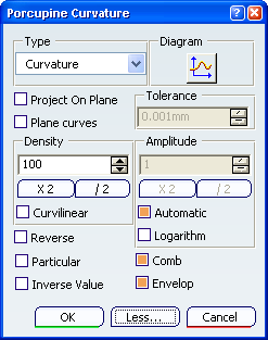
Open the analysis dialog box:
View the comb analysis on a surface and then on a curve:
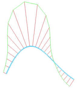
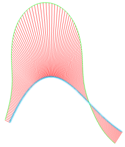
- Select a surface in the 3D area.
- If you select the surface, the porcupine comb shows the curvature on each boundary of the surface.
- If you select a specific boundary, the comb is displayed
only on this boundary.
Ensure the Geometrical Element
Filter selection mode is active from the User Selection
Filter toolbar (this mode lets you select sub-elements).
- If you select the surface, the porcupine comb shows the curvature on each boundary of the surface.
- Select a curve in the 3D area.
The porcupine comb shows the curvature of the curve.
- In the Type area of the dialog box, select Radius.
The porcupine comb now shows the radius of the curve.
- Select a surface in the 3D area.
Adjust the characteristics of the porcupine comb:
- In the Density area of the dialog box, adjust the number of spikes in the comb by using the arrows in the spin box or by clicking X2 and /2.
In this example the density of the spikes has been increased.
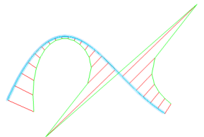
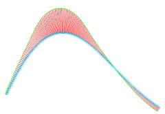
- In the Amplitude area of the dialog box, clear the Automatic check box and then adjust the length of the spikes in the comb by using the arrows in the spin box or by clicking X2 and /2.
In this example the amplitude of the spikes has been decreased.
Notes:
- Adjusting the density of the spikes is particularly useful when the geometry is too dense to be read but the resulting curve may not be smooth enough for your analysis needs.
- When Automatic amplitude is selected, the length of the spikes is optimized so that even when zooming in or out, the spikes are always visible.
- In the Density area of the dialog box, adjust the number of spikes in the comb by using the arrows in the spin box or by clicking X2 and /2.
Use the Particular option to display the minimum and the maximum points.
You can right-click on any of the spikes and select Keep this Point to keep the current point at this location. A Point.xxx appears in the specification tree. If you select the Particular option, you have access to more contextual commands:Important: - Inflection points are displayed only if Project on Plane and Particular options are selected.
- The Inverse Value option displays the inverse value in Radius when the Curvature option is selected, or in Curvature when the Radius option is selected. This option does not recalculate Max and Min type values, it displays only the inverse values and Max and Min location for the selected type are still displayed.
Important: All these contextual commands are applicable not only to the curve where you right-click the spike, but to all the curves involved in the analysis. View a curvature diagram:
- In the Diagram area of the dialog box, select Display diagram window
 .
.The 2D Diagram dialog box appears.
The curvature amplitude and parameter of the analyzed curve are represented in this diagram.

Important: - In the curvature graph, the X axis abscissa is curvilinear when Curvilinear is enabled in the Porcupine Curvature dialog box, otherwise the X axis abscissa is parametric. When X axis abscissa is parametric, its range is not necessarily between 0 and 1.
- The X axis abscissa values are independent of the selected type of curvature analysis, Radius or Curvature.
When analyzing a surface or several curves, you can use different options to view the analyses.
For example, when analyzing a surface, by default you obtain this diagram, where the color of the curves in the 2D Diagram dialog box match the ones on the geometry.
- In the Diagram area of the dialog box, select Display diagram window


Notes:
- The Reverse analysis is opposite to that which was initially displayed. This is useful when, from the current viewpoint, you do not know which way the curve is orientated.
- Project on Plane option applies a curvature signature due to the curvature analysis projection.
- In case of clipping, you may want to temporarily modify the Depth Effects' Far and Near Limits. See Setting Depth Effects in Infrastructure User Guide.